Compressions
One challenge when dealing with big data is not to "miss the wood for the trees". The task is to filter the crucial information from terabytes of data.
Of course, the question can now be raised as to why so much data is collected if only a fraction of it is to be retained in the end. In connection with the high-frequency analysis in Optimizer4D, this is explained quite simply:
The sampling rate at which a signal is sampled is directly related to the maximum observable frequency: For physical/mathematical reasons, it is not possible to detect frequencies that are higher than half the sampling rate.
For high frequencies that we want to observe, we therefore need a sampling frequency that is at least twice as high. In order to be able to observe signals up to 50Mhz, we must therefore sample at a frequency of at least 100Mhz.
This alone means 200MB per second if we assume 16 bits per value.
After the FFT conversion, the data rate can be even higher, depending on the parameterisation.
The trick lies in processing the data step by step, extracting the relevant information and then compressing or summarising the data.
To achieve this, our software can apply different compression approaches directly to the data stream in real time. The trick is to apply the compression only after the frequency conversion so that we do not limit our observable bandwidth.
In addition, with our graphical programming tool, real-time analyses can be compiled with just a few clicks and applied to the data during the measurement.
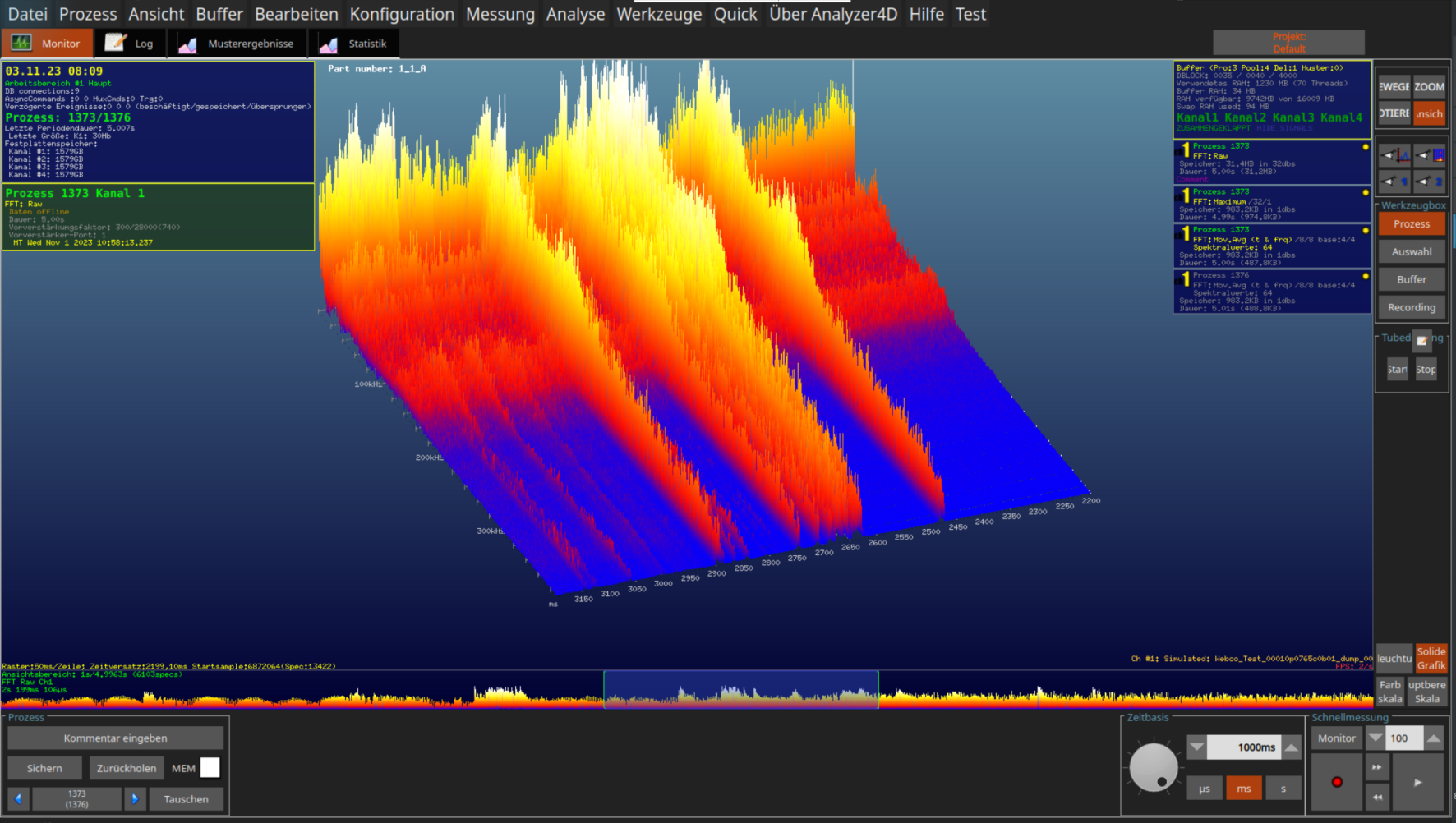
Raw signal
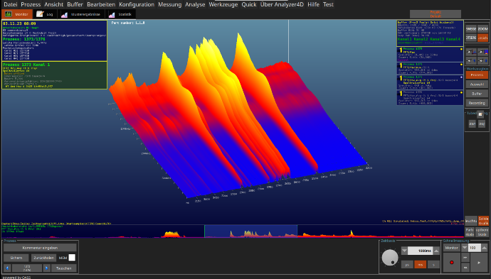 Real-time compression
Flexibility and customisation
Intermediate results and further data processing stages can be saved from here in SQL databases, for example.
For maximum flexibility, special analyses and data transformations can be integrated directly into the real-time analysis using Python.
Measurements that appear conspicuous can be marked for longer storage in raw format so that they can be inspected later.
Our pipeline
- High-resolution Digitisation in the MHz range
- FFT calculation in real time to observe the full frequency bandwidth
- Pre-filtering of the FFT display
-
- Band filter
- Smoothing
- Compression
- Real-time analysis with our operator network
-
- Extension with Python
- Saving results in database for long term data retention
- Marking conspicuous measurements for long-term storage
-
- Unremarkable data is discarded after a few hours discarded
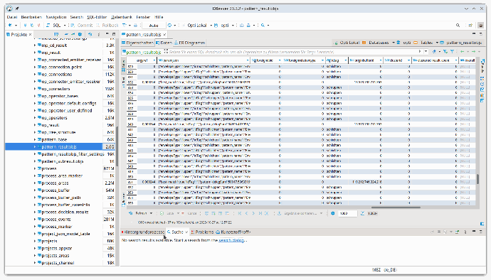
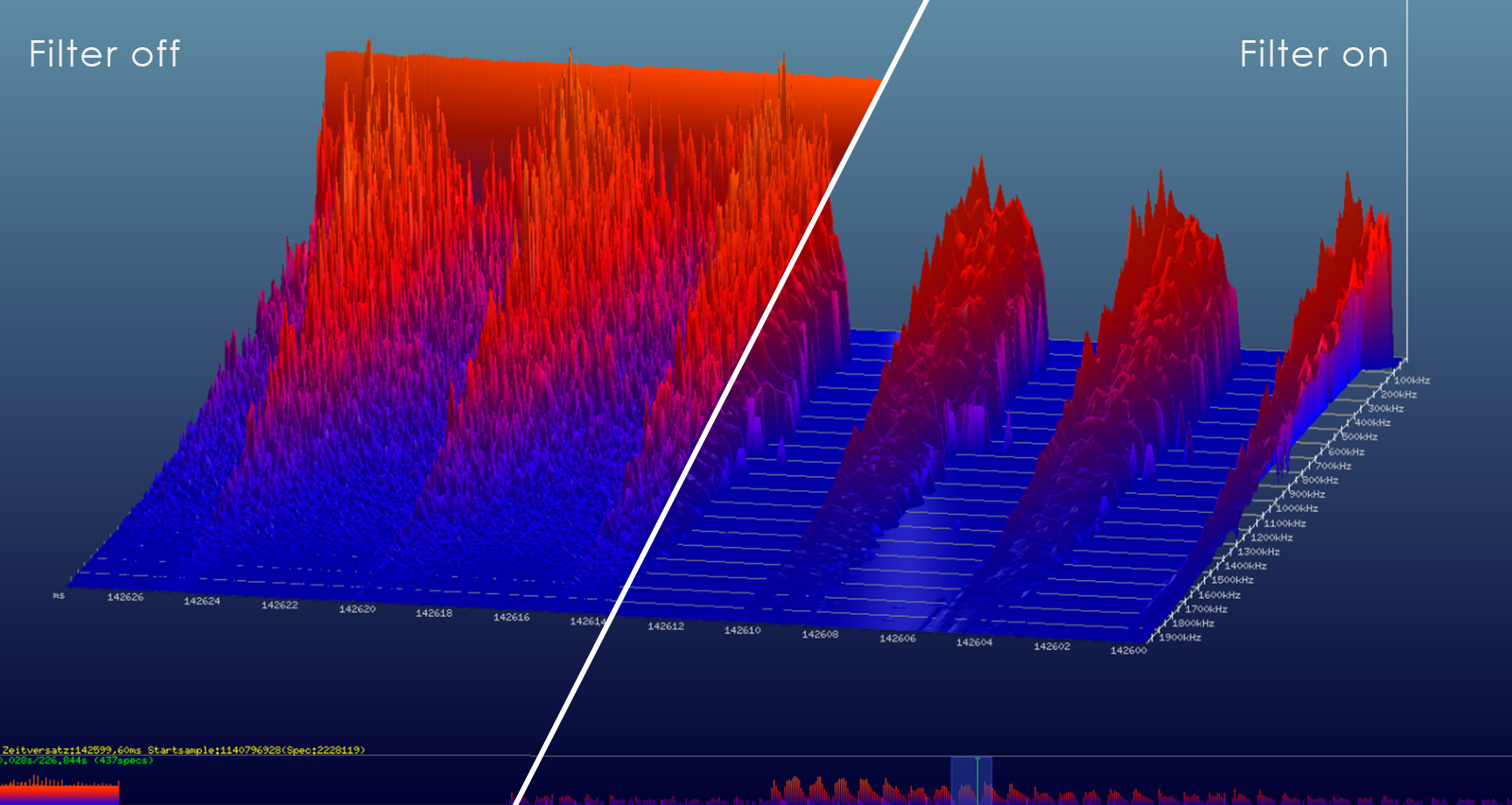
Filtering the data in our process landscape
Compression via dimensional reduction
The classic approach to data compression described above is contrasted with more modern approaches that realise data compression via dimensional reduction. Here we present a brief summary of two possibilities.
The first option for dimension reduction is the so-called Singular Value Decomposition (SVD). The SVD takes the measurement data as a matrix and calculates a decomposition into three components whose dimensionality is significantly lower than that of the original measurement data. The measurement data can be restored by multiplying these three components. The quality of the reconstruction increases depending on the degree of dimensionality reduction, also known as the rank. A low rank results in a strong compression of the data, but also leads to a higher reconstruction error. If the rank is set to maximum, the data can be reconstructed without errors. However, the data consumption saved is minimal.
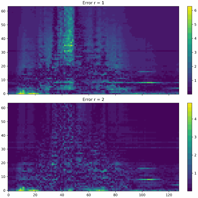
The two figures below show the error of a data reconstruction at rank 1 and rank 2 respectively. It can be seen that the reconstruction error at rank 1 is strongly concentrated in certain regions of the measurement data, whereas the error at rank 2 is much smaller and more evenly distributed. How strong the compression should be and how small the reconstruction error may be depends entirely on the application. The rank of the SVD must be selected according to the requirements.
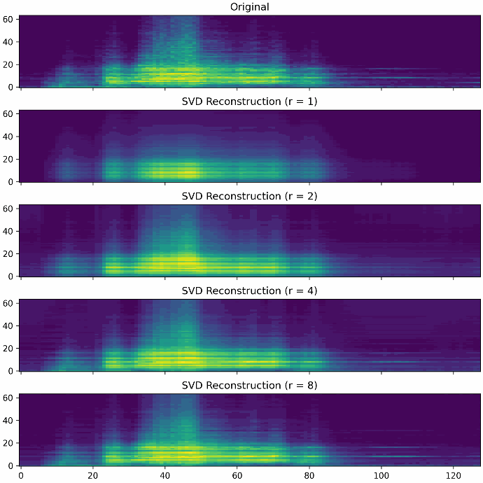
The figures below show different reconstructions with the ranks 1, 2, 4 and 8. It can be clearly explained that with a higher rank more subtleties of the original measurement data are reconstructed.
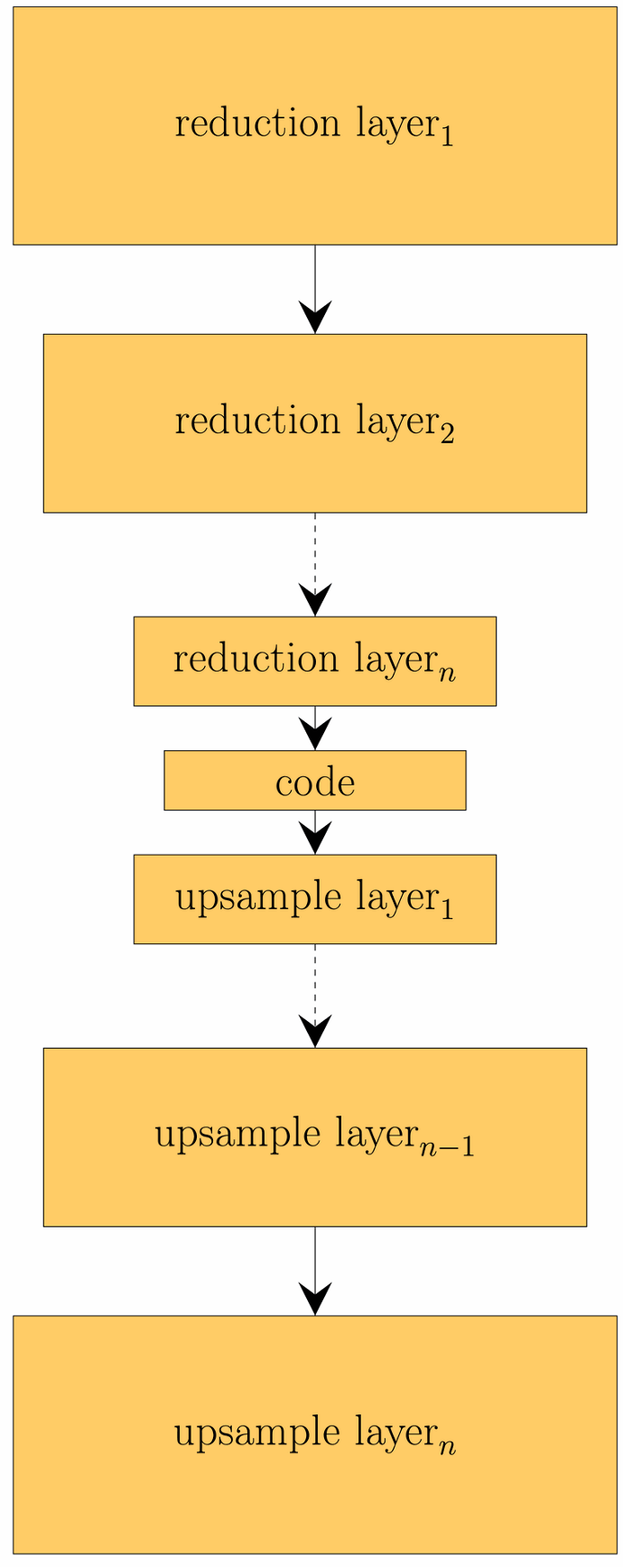
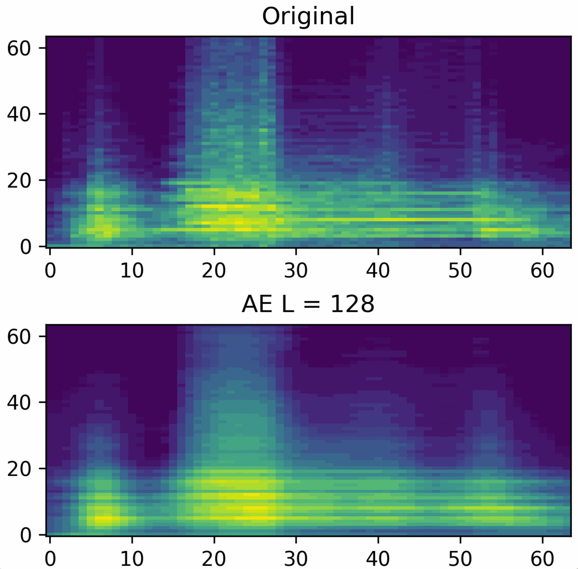
As an alternative to SVD, dimension reduction can also be implemented using an autoencoder architecture, for example. An autoencoder is a special form of neural network that consists of an encoder and decoder.
The encoder reduces the dimensionality of the input data and maps it to a code that represents the data. The input data can be reconstructed from a code via the decoder. This reconstruction is generally subject to errors. The idea behind the learned code is that it represents complex relationships between the input data. This is an advantage over SVD, which can only represent linear relationships. The figure below shows a reconstruction using an autoencoder.
The dimension-reduced representations can be used not only for compression, but also for further calculations.machine learning