Machine Learning
The in-line monitoring of components or machines often presents us with unknown challenges. When analyzing our measurement data, we are repeatedly confronted with an abundance of information. In the case of complex data with correlations that are difficult to interpret, it is possible to correlate machine events qualitatively with the data using a great deal of experience of the manufacturing process from which the data originated and to extract these qualitative characteristics using analytical methods in complex, multi-stage development steps. However, this requires that the data always fulfill these qualitative characteristics and do not change in their characteristics. Otherwise, the complex development steps must be repeated in order to adapt to changes in the data.
In the long term, this approach is very maintenance-intensive and labor-intensive. In the worst case, it requires long-term support or redevelopment. In order to adapt to the circumstances and extract as much information from the data as possible, we use common machine learning methods using Python and established libraries such as Pytorch to correlate our data with the data of the component or machine to be monitored. The extracted features are generally more robust and are summarized by the resulting models in such a way that changes in the signal characteristics can also be mapped and noticed using this approach.
Machine learning for gear grinding and other complex industrial applications
The aim of quality assurance is to ensure the consistently high quality of the manufactured parts. There are two typical processes:
- Checking the manufactured parts for known defect patterns
- Monitoring the production process for process changes
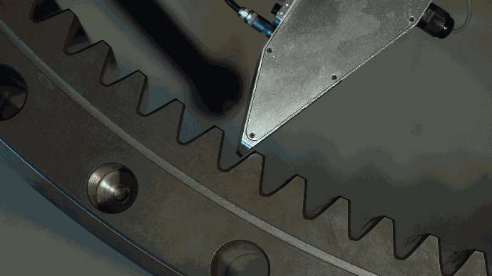
With our structure-borne sound measurement system, it is possible to listen to the machine at work. In this way, we can detect problems directly where they arise and point out process changes at an early stage. We sample the signal several million times per second and thus obtain a high-resolution measurement image of the process itself. A digitized image of what is happening in the process. We create a digital twin without a CAD model - not of the component, but of the manufacturing process.
A common quality assurance procedure is to monitor a characteristic value for violations of warning and action limits. This approach is based on the assumption that the monitored characteristic value remains constant and is largely free of variation.
The reality is different: Manufacturing processes are subject to a variety of influencing that have an impact on production:
- Temperature fluctuations
- Starting material
- Tool wear
- Pre-processing steps
- Etc.
The more sensitive the measuring device, the more clearly it perceives the effects of such factors. However, to ensure the highest quality, you naturally want to use a highly sensitive measuring method and the narrowest possible tolerance limits. This requirement means that even the smallest changes in the environment lead to rejects.
In practice, therefore, the limit values must be adjusted so that they cover all normal process fluctuations that do not yet result in a reduction in quality.
We have developed a concept that allows us to measure and evaluate with high sensitivity despite fluctuating production conditions. We use machine learning to follow the process fluctuations.
The usual approach would be to train a model on the basis of 100,000 measurements and the associated assessment (good/bad) in order to automatically derive the assessment from the measurements.
However, this approach has several catches: Let's assume that we only need 5000 measurements of defective parts and a defect rate of approx. 1‰, then that amounts to 5 million parts that need to be evaluated and checked for defects. Have you ever tried to get a reliable and complete component defect analysis for just 100,000 parts? And are you sure that you have mapped the usual process fluctuations during data generation?
We use machine learning to understand the relationship between environmental parameters and structure-borne sound signature. More precisely, we observe, analyze and learn from this. This means that after a training phase, we can predict which structure-borne sound measurement image we expect. The good thing about this is that we receive countless data for this training - with every part that is manufactured, we gain new insights into machine and environmental parameters and their effect on the measurement result.
Once the expected result has been identified, the limits can be adjusted accordingly. This results in variable tolerance limits that can adapt to the expected changes. Or to put it another way: We transform the measurement results so that known process changes are factored out and focus on the deviations from the expected!
In the Video you can see these relationships.This was specifically about changes to machine parameters that have a strong impact on the measurement result. Each individual image of the changing 3D landscape represents the FFT structure-borne sound signature of the production of a component. Over time, you can therefore see the process changes in fast motion. Due to the process-immamental variations, it would not be possible to assess the production quality with the conservative QA approach of fixed limit values.
Of course, this methodology is not limited to structure-borne sound or grinding processes: Machine learning is geared towards recognizing structures and correlations in data. Complex relationships between the environment and the manufacturing process or its measurement can be trained and learned through observation.
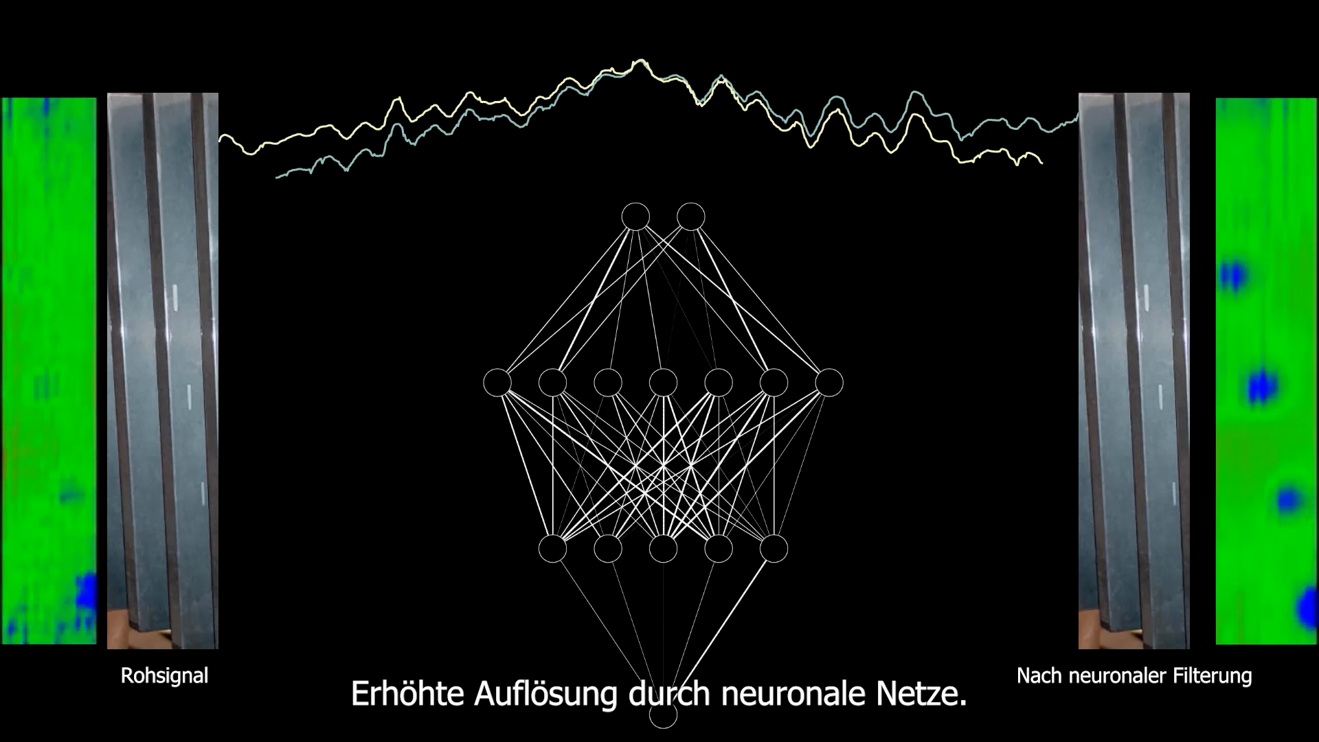 Comparison: Raw signal vs. signal after neuronal filtering.
Machine learning in the detection of grinding burns
Our fully automated grinding burn test can detect and display defective areas in the component. The grinding burn test is carried out as a special anomaly monitoring system. It searches for material areas that deviate from the rest of the material.
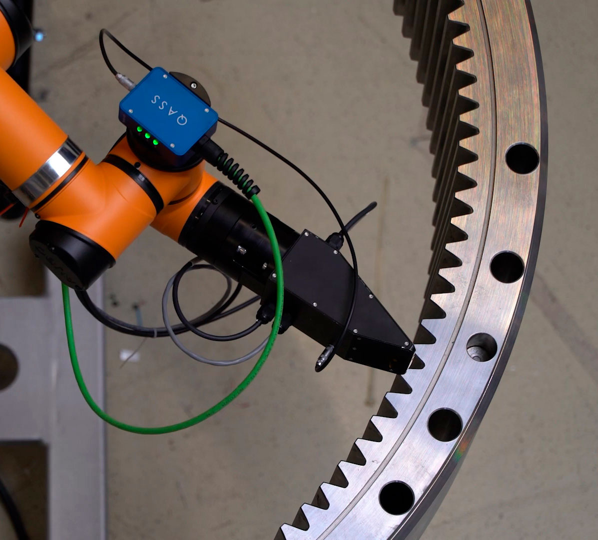
The method used is based on Barkhausen noise. The material is magnetically excited and we observe the resulting Barkhausen noise in the ferromagnetic material. For reproducible and precise measurement results, we carry out the grinding burn test with a special robotic system in which the sensor is guided over the material surface at a distance of approx. 1 mm. The measurement signal depends on various influencing variables, e.g. frequency, excitation intensity, material composition, residual stresses, but above all the distance
With the help of several distance sensors, we record the distance and sensor tilt for each measured value. This involves not only the vertical distance, but also tilting of the sensor.
As described above for grinding, we also collect an additional influencing variable of the measurement here. We train neural networks with which we learn the relationship between sensor tilt, component geometry and distance.
Any mechanical fluctuations in the robot system can therefore be automatically taken into account and compensated for in the analysis. Thanks to the non-contact measurement, the products are measured quickly and non-destructively, and we then compare the measurement result obtained with the expected results for the evaluation. The neural network provides us with the usual measured value for the current distance so that we can differentiate the influence of material anomalies on the distance. This gives us maximum sensitivity when searching for defective areas.
Data Augmentation
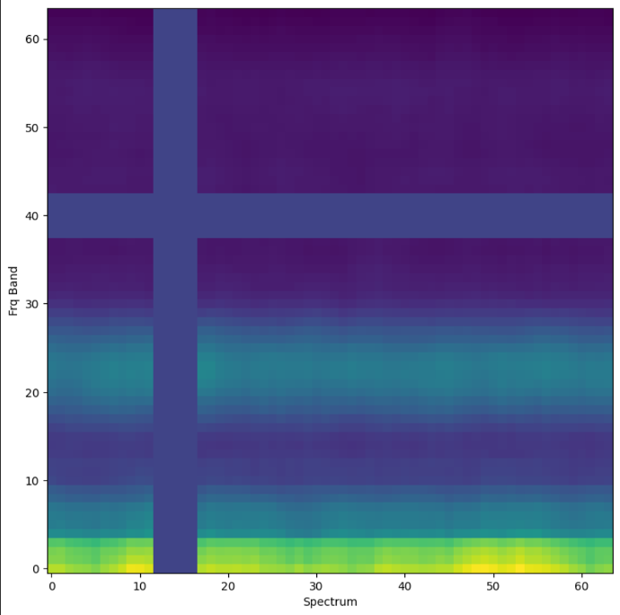
A general challenge in the application of machine learning models is their transferability. If you want to apply the model after training to a new data set that differs in some way from the data from the training, you often run into the problem that the model cannot cope well with these changes. As a consequence, the quality of the model output is correspondingly lower. To counteract this, data augmentation techniques are often used, i.e. the artificial expansion of our data through targeted manipulation. This can be, for example, changing the basic energy level of the measurement, adding noise to the data or masking certain time or frequency ranges (see figure). This counteracts the memorization of certain data properties (overfitting) and thus enables better generalization capability.
Singular value decomposition for clustering high-dimensional data
When recording large amounts of data, we are repeatedly confronted with the task of extracting and grouping qualitative and quantitative properties, such as certain signal characteristics, from the data. Unsupervised learning methods, in particular clustering, are generally used for this purpose.
The calculation of clusterings for our data is generally challenging due to the high dimensionality (Curse of Dimensionality). A process section of 64 spectra on the time axis with 64 frequency bands already results in a data point with 4096 dimensions. In addition, the non-uniform length of the recordings means that many methods are not readily applicable.
To tackle both challenges at the same time, we use the calculation of a Singular Value Decomposition (SVD). This considers a process section as a matrix and decomposes it into three components, which then provides a uniform form of significantly lower dimensionality (often < 10 in the application).
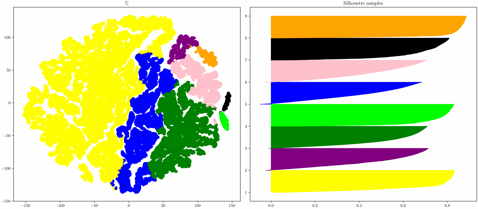
The image on the left shows a calculated clustering based on a component of the SVD. The colors correspond to the individual clusters.
The "silhouette scores" for each individual process section of the clustering are shown on the right, which describe how well the clusters are delimited from each other. Silhouette scores greater than zero indicate that the respective element is well integrated into its own cluster. Scores less than zero, on the other hand, indicate that the assignment of the element was not optimal and that it would be better to assign it to a different cluster.
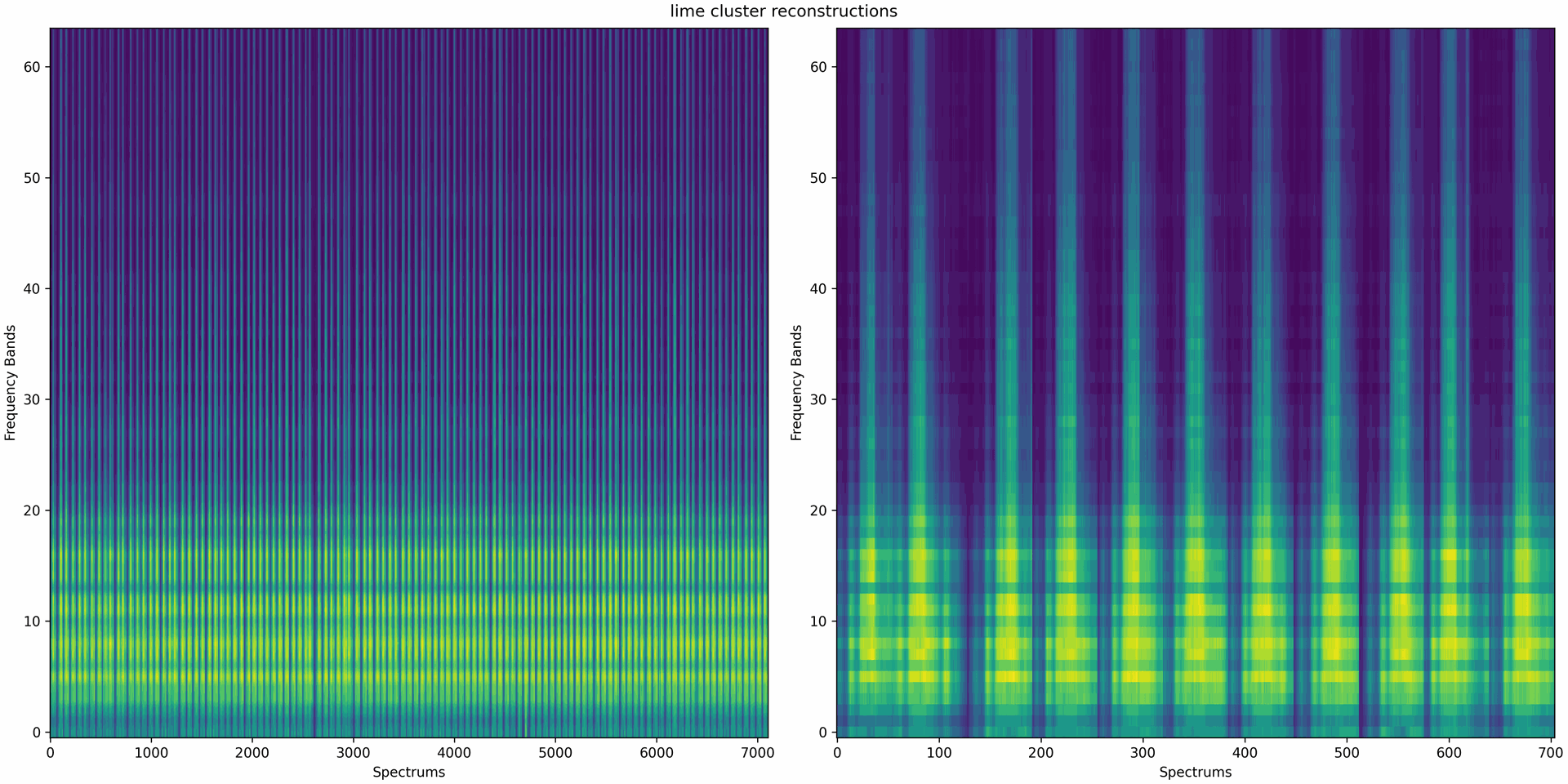
The left-hand image shows 100 random process sections from the light green cluster. The right image shows a section of the left image with 10 process sections. The homogeneous appearance of the randomly selected process sections shows that the clustering of the SVD components successfully combines similar process sections.
The dimension reduction property of the SVD can also be used for data compression.
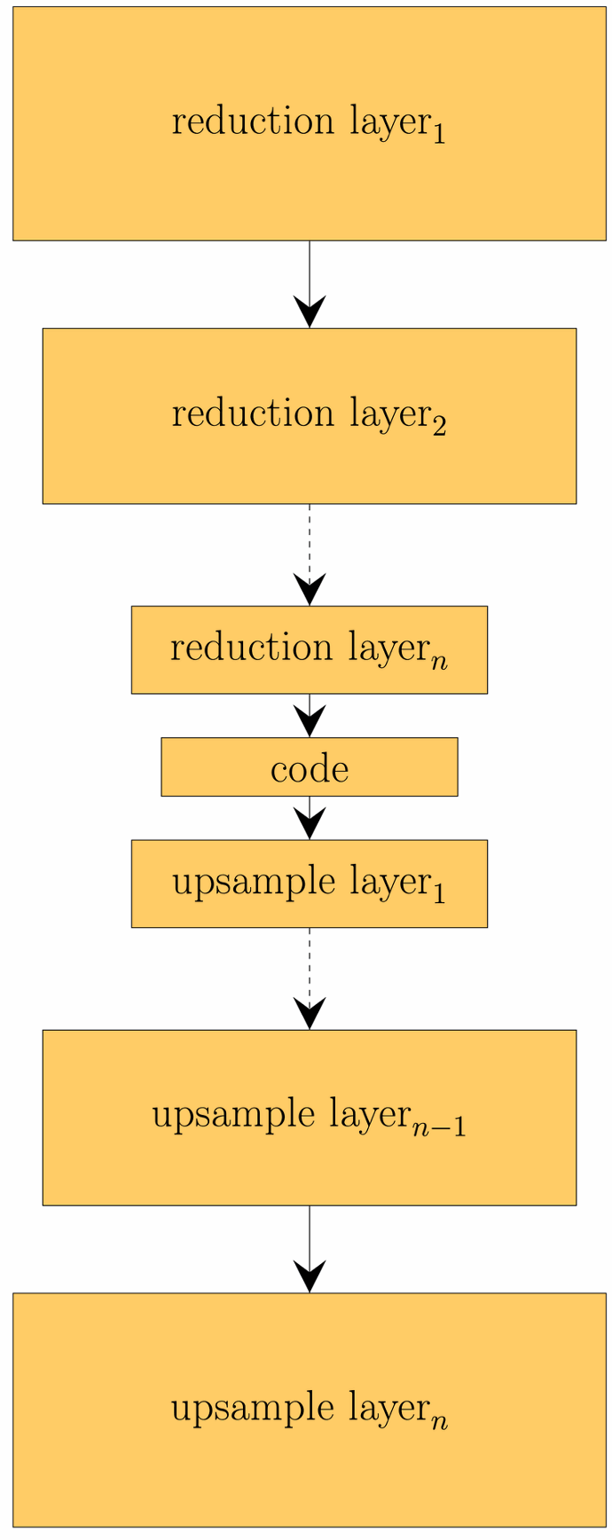
Dimension reduction via autoencoder
As an alternative to the SVD considered above, the dimensionality of the data can also be reduced using a so-called autoencoder. An autoencoder is a special form of neural network that consists of two parts: an encoder and a decoder. The encoder reduces the dimensionality of the input data and maps it to a code that represents the data. The decoder can be used to reconstruct the input data from a code. This reconstruction is usually subject to errors. The idea behind the learned code is that it represents complex relationships between the input data. This is an advantage over SVD, which can only represent linear relationships.
Like the SVD, autoencoders can also be used for data compression.
Splitting processes into signal sections with RBF Kernel
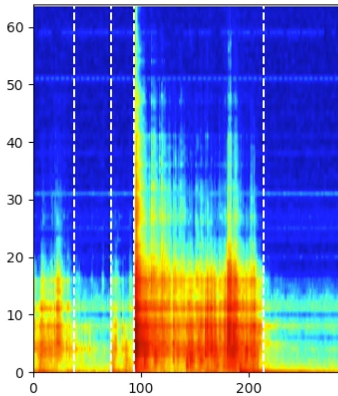
A process can usually be subdivided into several work steps, which are considered separately depending on the application. If such a division does not already result from the machine communication or is still fine enough, a technique is required to divide the process solely on the basis of the measurement signal. Since our data usually has several frequency bands, it is very important to consider how the frequency bands behave with each other.
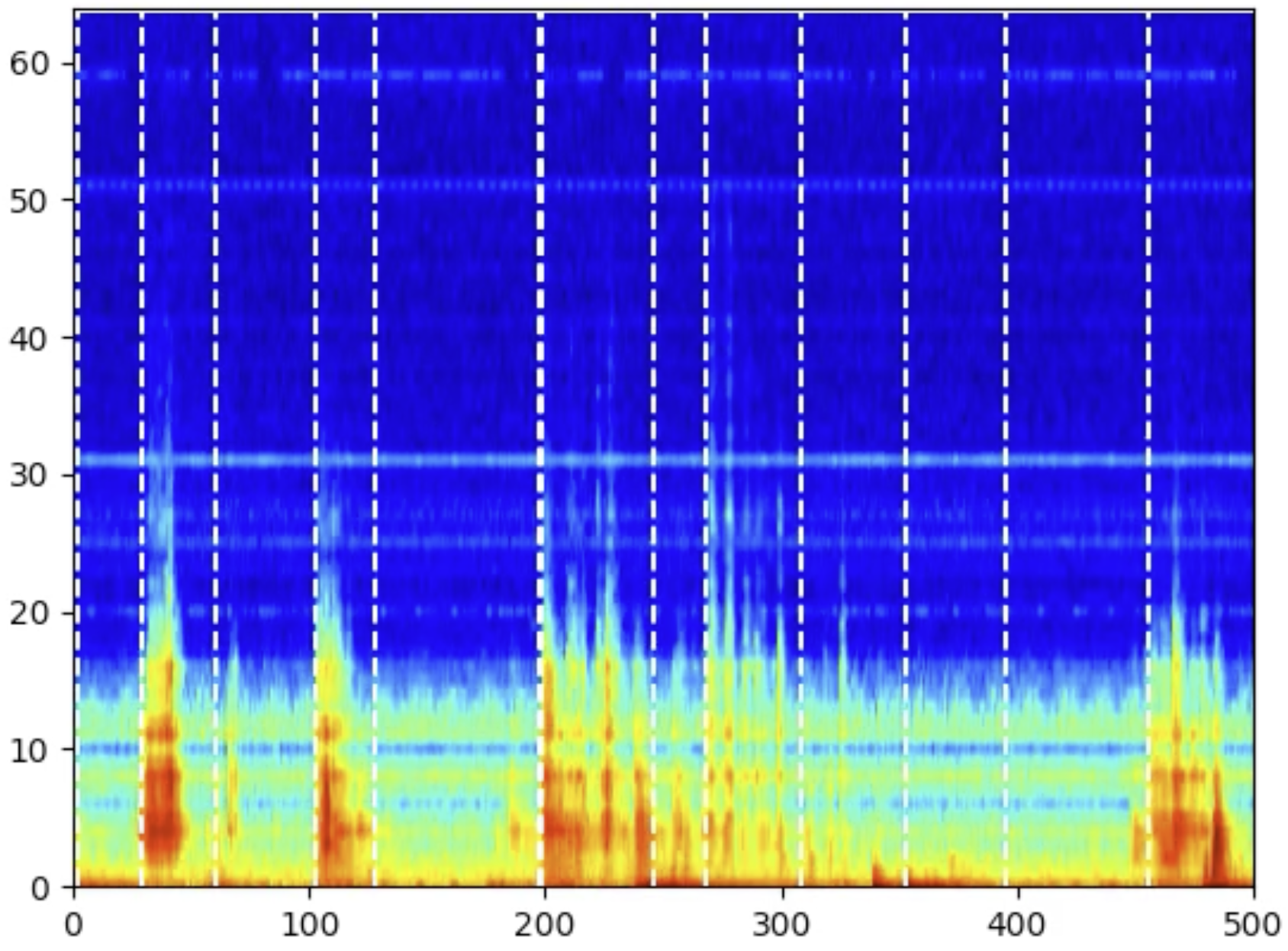
The problem here is that there can theoretically be an infinite number of combinations of how the frequency bands are viewed. A mathematically elegant and widely used technique to represent all these combinations in a compact way is the use of the Radial Basis Function Kernel (RBF Kernel). This makes it possible to view all combinations without actually having to calculate them. The kernel can be understood as a distance measure in a transformed data space that encodes the information of all dimensions of the data. If we then use the RBF kernel to determine how similar successive spectra are, we can identify the points in time in the signal at which the signal characteristic changes and thus a new signal section begins. In each of the two figures, we see a process section including the points at which the signal is split, indicated by the white lines.